USGS Digital Raster Graphics
U.S. Geological Survey - Mid-Continent Mapping Center
July, 1997
A common question about U.S. Geological Survey (USGS) digital raster graphics is "how can I remove the map collars and join multiple quadrangles together?" The question does not have a simple answer because of the characteristics of USGS quadrangles.
Quadrangle neatlines are defined by lines of latitude and longitude, so quadrangles are not rectangles on their published projections. But digital raster images are necessarily perfect rectangles. Clipping a digital neatline is therefore not directly comparable to cutting a paper map with scissors. Paper maps are oriented with the neatlines approximately parallel to the paper edges, but digital data sets are oriented so that the image coordinates are aligned with a selected plane ground coordinate system, or grid. Grids generally are not parallel to the quadrangle boundaries, so displayed digital data sets may appear tilted.
Digital data serve different purposes than paper maps, and therefore may be placed on different projections. Most USGS digital products are projected on the Universal Transverse Mercator (UTM), regardless of the projection of the corresponding topographic map.
The U.S. Geological Survey (USGS) uses a variety of projections for its maps. Projection decisions always represent tradeoffs between different types of distortion and convenience. The goals of low distortion, product standardization, and end user ease of use are not perfectly compatible. For each cartographic product, the USGS attempts to strike a reasonable balance between these conflicting goals.
Of particular interest to many users are digital raster graphics (DRG). A DRG is a digital image of a paper map. The projection change to Universal Transverse Mercator (UTM) creates a conflict between the data and the map collar information, and in some cases visibly changes the appearance of the map image. These changes can be confusing to users.
This paper explains the characteristics of Transverse Mercator projections, the relationship of plane grids to USGS map cells, and the reasons DRG's and other USGS digital products are projected on the UTM.
There are three types of developable1 surfaces onto which most USGS maps are projected. They are the cylinder, the cone, and the plane (Snyder, 1987, p. 5). This paper discusses two varieties of cylindrical projections: regular and transverse cylindrical.
If a cylinder is wrapped around the globe so that its surface touches the Equator (fig. 1), the meridians of longitude can be projected onto the cylinder as equally spaced straight lines perpendicular to the Equator. The parallels of latitude are also straight lines, parallel to the equator, but not necessarily equidistant (Snyder, 1987, p. 5).
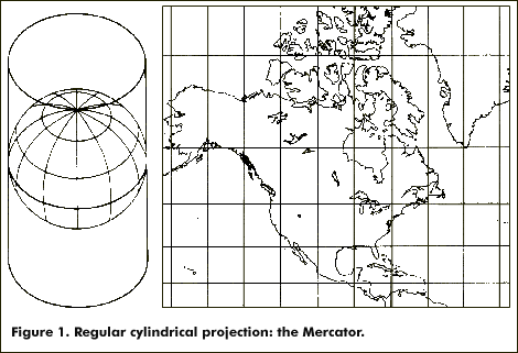
The Mercator (fig. 1) is the best known regular cylindrical projection. The Mercator was designed for sea navigation because it shows rhumb lines2 as straight lines. Unfortunately, it is often and inappropriately used for world maps in atlases and wall charts. It presents a misleading view of the world because of excessive area distortion (Snyder and Voxland, 1989, p. 10). The Mercator shows meridians and parallels as straight lines. Regular cylindrical projections are the only commonly used projections that show both meridians and parallels as straight lines.
Setting the axis of the cylinder perpendicular to the axis of the Earth results in a transverse cylindrical projection (fig. 2).
In a transverse cylindrical projection, the point of tangency between cylinder and globe is a meridian, or line of longitude, called the central meridian. Neither parallels nor meridians are straight lines, but rather are complex curves (fig. 2).
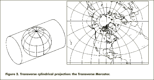
The best known transverse cylindrical projection is the Transverse Mercator. The Transverse Mercator was invented by Johann Lambert (1728-77) (Snyder, 1987, p. 48), even though it is named after Gerardus Mercator (1512-94). Figures 1 and 2 illustrate that the Mercator and Transverse Mercator projections are dissimilar.
On a Transverse Mercator, the central meridian (the central north-south straight line in figure 2) is the line of true scale3. This makes the projection appropriate for areas with long northsouth extent and narrow east-west extent.
The UTM projection and grid were adopted by the U.S. Army in 1947 for designating rectangular coordinates on large-scale maps for the entire world. The UTM is a Transverse Mercator to which specific parameters, such as standard central meridians, have been applied (Snyder, 1987, p. 57). The Earth, between latitudes 84° N. and 80° S., is divided into 60 zones, each 6° wide in longitude.
Calculations to relate latitude and longitude to positions on a map can become quite involved. Rectangular grids have therefore been developed for the use of surveyors. In this way, each point can be designated merely by its (x,y) coordinates. Of most interest in the United States are two grid systems: the UTM grid and the State Plane Coordinate system (SPCS) (Snyder, 1987, p. 10)
Grids are appropriate even when powerful digital computers are available. In large raster images, it is convenient to arrange the rows and columns of image pixels in alignment with an accepted surveying grid. Most image display software depends on a simple relationship between image coordinates and screen coordinates.
Grid systems are normally divided into zones so that distortion and variation of scale within any one zone are kept small. Zones of the UTM are bounded by meridians of longitude, but for the SPCS, State and county boundaries are used. In both the UTM and the SPCS, all USGS quadrangles within a given zone can be mosaicked exactly (Snyder, 1987, p. 57), but two adjacent quadrangles that belong to different zones cannot be mosaicked without reprojection. This is true of both printed paper maps and digital cartographic products.
Graticules
A map graticule is a network of lines representing parallels and meridians.
Figure 3 illustrates the relationship between a graticule and a grid of plane coordinates4. The figure shows that grid lines usually do not coincide with graticule lines except for the central meridian and the Equator (Snyder, 1987, p. 10). Regular cylindrical projections are an exception, because parallels and meridians are straight lines on these projections.
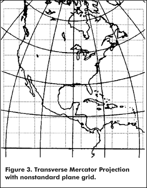
Figure 4 is part of a diagram showing the locations of UTM zones.
Although figure 4 is a map of UTM zones, it is not a Transverse Mercator map. The continent outlines and graticule in figure 4 are on a regular cylindrical projection (Equidistant Cylindrical). The meridians that define UTM grid zones are therefore shown as straight lines.
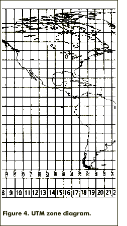
Map users who are not familiar with projection characteristics sometimes infer from such a diagram that UTM grids correspond to the graticule. This is not the case. UTM grid lines actually have a relationship to the graticule similar to that illustrated in figure 3. The lines in figure 4 are graticule lines that define the boundaries of UTM zones and that happen to be straight because of the projection they are drawn on; none of these zone boundaries match UTM grid lines.
USGS standard quadrangle maps are bounded by parallels and meridians. The standard USGS topographic map series are 7.5' x 7.5' (1:24,000 scale), 60' x 30' (1:100,000 scale) and 2° x 2° (1:250,000 scale).
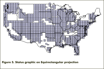
USGS map indexes and status graphics often show quadrangles on regular cylindrical base maps. Figure 5 is a status graphic from a USGS web page5. The projection for this graphic was selected so that all quadrangles would be rectangular and of equal size. Map users who are not familiar with map projections might infer-incorrectly-from this diagram that USGS quadrangles are rectangular.
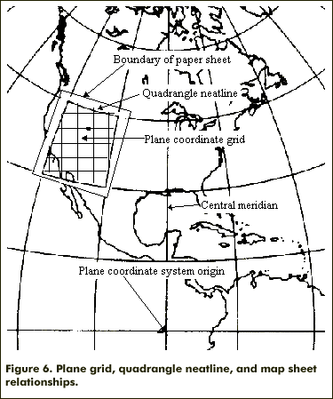
To illustrate the real relationship between USGS quadrangles and plane coordinate systems, suppose there were a series of standard maps for North America, 15° x 15° in size, projected on the Transverse Mercator projection of figure 2. Figure 6 shows how a quadrangle west of the central meridian would be defined.
Transverse Mercator would not really be used for areas as large as those shown in figure 6, but the exaggerations caused by the large area illustrate several things about the relationships between USGS quadrangle maps, the graticule, and plane coordinate systems:
Consider a digital cartographic data set that covers the same geographic area as a quadrangle. A DRG is the easiest to visualize because it is a scanned image of a quadrangle map, but these comments apply to digital orthophoto quadrangles (DOQ) and any other quadrangle-based raster images7.
At the physical file level, a DRG is a simple raster image. That is, it has these characteristics:
A DRG therefore has the geometric characteristics of a projected plane grid, not those of a graticule. For this reason, it is useful to align the rows and columns of a DRG with the rows and columns of a plane ground coordinate system. This makes the relationship between image coordinates and ground coordinates arithmetically simple.
Figure 7 shows the boundaries of digital data sets associated with a Transverse Mercator map. The minimum bounding rectangles in the figure are two potential data set boundaries. The edges of the data set align with the plane grid, not with the graticule that defines the quadrangle boundaries. The DRG data set cannot align with or match a USGS quadrangle exactly, because the quadrangle boundaries do not form a rectangle8. The actual extent of a DRG data set is usually somewhere between the two minimum rectangles shown in figure 7.
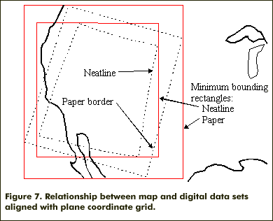
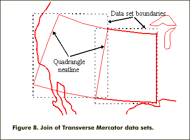
Aligning the file coordinates with plane ground coordinates has a significant visual side effect. When displayed on a screen, the map looks tilted (figs. 7 and 8). The amount of the tilt depends on the projection and the distance of the quadrangle from the central meridian, but it is frequently enough to be visually obvious.
The fact that the data set is aligned with a plane grid rather than the graticule does not prevent adjacent quadrangles from being joined. Quadrangles within the same plane coordinate zone join correctly, just as their paper counterparts do.
However, joining the edges of raster data sets is different than joining quadrangles. Figure 8 illustrates that clipping a digital data set at the map neatline is not directly analogous to cutting a paper map with scissors. Digital image files, unlike pieces of paper, are necessarily rectangular.
How, then, does a user mosaic multiple data sets into one image? There are at least two general answers to this question: software manipulation and data repackaging.
Some display software can render selected parts of an image transparent, so that images can be laid on top of each other without masking features of interest.
For example, the area outside the neatline in a DRG image can be identified and made transparent. Two or more images can then be placed in their correct relative positions in a new file or a virtual display space. The details of how to do this depend on the design and capabilities of individual software packages.
Because USGS digital data are georeferenced, the data files contain the information needed to automate the process of joining digital quadrangles. A sufficiently powerful geographic information system (GIS) can hide some or all of the details of joining quadrangles from the end user.
The worst case is when adjacent quadrangles are in different plane coordinate zones. One or both of the data sets must then be reprojected to a common zone. This can also be automated, although it requires relatively powerful software.
Data Repackaging
A second way to join quadrangles is to redefine the data. This can be thought of as a preprocessing step to make it easier for software to join quadrangles.
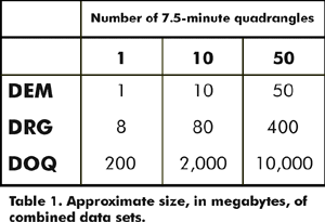
The simplest example of repackaging is to join a number of quadrangles with the software techniques described above and then save the result as a new data file. The obvious drawback is that data files can become very large (table 1). For state-sized areas, it is doubtful that such files can even be created.
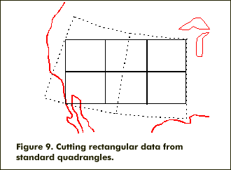
A better solution is to join several quadrangles, cut perfectly rectangular pieces from the combined data, and store the cut pieces as new data sets (fig. 9). In this way, physical files can correspond exactly to a selected plane ground coordinate system. For example, each data file might contain the data for a 10,000meter square UTM cell. Preprocessing the data in this way makes run-time calculations simple and fast, and therefore makes it easier to establish (for example) large image databases that appear seamless to the end user.
Most USGS 7.5-minute published quadrangles are projected on the Lambert and Transverse Mercator projections of the SPCS. But most 7.5minute digital products are projected on UTM. Why does the USGS use different projections for products that cover the same geographic cell and have similar content?
There is no such thing as a perfect projection. All map projections represent tradeoffs between different types of distortion. Selecting a projection requires consideration of several factors, one of which is the intended use of the map.
Printed paper maps and digital data files are not used for exactly the same things. Some of the differences include the following:
When designing the DRG, the USGS considered two projection options: retain the projection of the published map or change the projection to the UTM. Each of these options had advantages and disadvantages. The decision to use the UTM was based on these factors:
There is no "best" projection for either a map or a digital cartographic data set. Projection decisions are always tradeoffs between desired map characteristics, which in turn depend on the desired use of the data. Projection decisions made many years ago for published paper maps are not necessarily the right decisions for corresponding digital data sets.
Having digital data does not remove the necessity to make projection decisions. It is possible to store digital data in unprojected form, but this only defers projection decisions until run time. Displaying or plotting a digital data set requires projecting the data to a flat surface. Because runtime projection is computationally intensive, the USGS has chosen not to distribute unprojected data for most digital data products.
The USGS projects most of its digital products on the UTM, in the belief that this will serve more user needs, more often, than any other single projection.
The USGS is responsible for maintaining nation wide data bases of cartographic data. USGS data products are some of the raw materials from which finished cartographic applications can be built, but they are not themselves consumer products. This is one result of deliberate government policy to avoid competition with private-sector cartography.
Snyder, John P. 1987. Map Projections--A Working Manual. U.S. Geological Survey Professional Paper 1395.
Snyder, John P. and Voxland, Philip M. 1989. An
Album of Map Projections. U.S. Geological Survey Professional
Paper 1453.

![]() U.S. Department of the Interior |
U.S. Geological Survey
U.S. Department of the Interior |
U.S. Geological Survey
URL: http://topomaps.usgs.gov/drg/mercproj/index.html
Page Contact Information: Contact USGS
Page Last Modified: Thursday, 11-May-2017 15:10:24 EDT
